The code is available here: https://github.com/MIC-DKFZ/nnUNet and the paper https://arxiv.org/abs/1809.10486.

0. Introduction

Each medical image segmentation task seems to require a specialized architecture of CNN. This results in many papers related to this topic with very specific details crafted for a specific task.

The authors claim that those handcrafted details aim to overfit, lack of generalization and the usage of UNet vanilla architecture suffers from a lack of adaptation.

The Medical Segmentation Decathlon was created to change this situation: the participants have to create segmentation architectures that generalize across 10 different datasets. Without any handmade customization from one dataset to another.

2. nnUNet (no-new-net)

2.1. Architecture

Medical Images are usually in 3D in DICOM (Digital Imaging and Communications in Medicine) or NIfTI (Neuroimaging Informatics Technology Initiative) format. nnUNet includes the 2D 3D and cascade UNet architectures with minor modifications.

Intuitively the 2D architecture appears sub-optimal for 3D images but in practice, I saw better accuracy in some cases. And the benefits are faster training/inference and lower memory footprint.

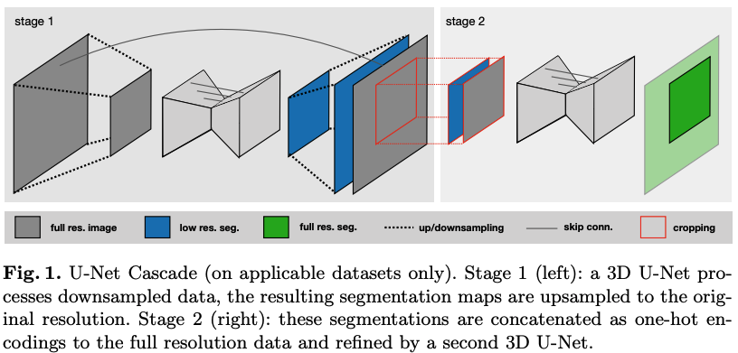
3D UNet is appropriate in most cases. However, with large images, because of memory constraints, the input 3D images are decomposed into patches. This can impact negatively the accuracy. For that reason, nnUNet includes also UNet Cascade.

In UNet Cascade, the first 3D UNet is trained on downsampled 3D images. Then the segmentation result is then upsampled and passed to a second 3D UNet which is trained on patches at full resolution. Figure 1 demonstrates this process.

To be able to manage the different sizes of images, the topology of the network is automatically adapted with respect to the dataset.

The 2D architectures start with a patch size of 256x256, a batch size of 42, and 30 feature maps for the highest layer (first layer of the "encoder"). Then these parameters are automatically adjusted with the median plane size of the input data. The architecture is also adapted to pool along each axis until the feature map size for each axis is smaller than 8.

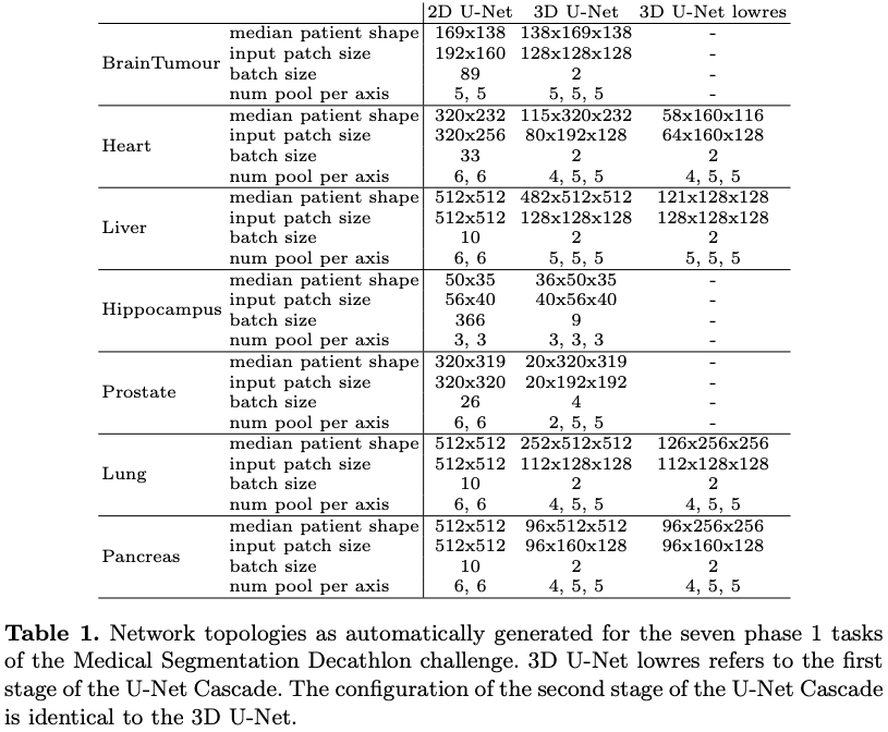
The 3D UNet starts with the same number of feature maps but with a patch size of 128x128x128 and a batch size of 2. Because of memory constraints (the paper's author has a GPU with 12 Gb of memory) the size of the input patch never exceeds $128^3$. As before the parameters are adjusted by looking at the median plane size. The pooling layers are set in the same way as the 2D architecture also. Another constraint is that the number of voxels ("pixels" in 3D) per optimization step (input patch size x batch size) is limited to 5% of the dataset. Table 1 gives an example of the parameters with respect to the dataset characteristics.

2.2. Preprocessing

The preprocessing operations are set automatically by the author's framework.

Cropping

In medical images, it is common to have large areas on the images that are 0s. Each image is therefore cropped to the region of nonzero values in order to reduce the size.

Resampling

The spacings between plans in 3D medical images are generally not consistent. Which is not something CNNs can handle. Therefore, each image of a dataset is resampled to the median spacing by using a 3rd order spline interpolation. The corresponding masks (ground truth) are resampled by using nearest-neighbor interpolation. For UNet Cascade a specific heuristic is used. All details are in the paper.

Normalization

There are 2 cases here. If the images from CT scan (computerized tomography), all values are collected and the entire dataset is normalized by clipping to the [0.5, 99.5] percentiles of these values. A z-score normalization is applied based on the mean and std of the values. If the dataset is from MRI (Magnetic resonance imaging) or other image modality, a simple z-score normalization is applied per image. Also if the cropping average size reduced the images by 1/4, then the normalization is done only by considering the values not contained in the segmentation masks equal to 0.

2.3. Training Procedure

The cost function is the addition of the dice and the cross entropy:

$\mathcal{L}_{total}= \mathcal{L}\_{ dice} + \mathcal{L}\_{CE}$

The original dice coefficient is:

$dice = \frac{2 TP}{2TP+FP+FN}$

With TP true positives, FP false positives, and FN false negatives.

The authors use a variation of this coefficient:

$\mathcal{L}\_{dc} = - \frac{2}{|K|}\sum\_{k \in K}\frac{\sum\_{i \in I}u_i^kv_i^k}{\sum_{i \in I}u^k_i+\sum_{i \in I} v^k_i}$

with $u$ is the softmax output of the network and $v$ a one host encoding of the segmentation mask (ground truth). Both have shape $I \times K$ with $i \in I$ the number of pixels in the training patch/batch and $k \in K$ the classes. Let's take an example of a good prediction for 2 classes and 1-pixel image:

$- \frac{2}{2} \times \frac{1 \times1}{1 + 1}= -0.5$

Considering the loss function earlier combining the cross-entropy and the dice, the best loss is therefore -1.

Adam Optimizer is used here with an initial learning rate of $3 \times 10^{-4}$ for all experiments. And epochs are defined as 250 training batches. To smooth the validation and training losses values, an exponential moving average is used. If no improvement on the training loss values (smoothed) by at least $5 \times 10^{-3}$ is observed for 30 epochs, the learning rate is reduced by a factor of 5. The training is stopped if not improvement above $5 \times 10^{-3}$ within 60 epochs is observed. But this rule doesn't apply if the learning rate is greater than $10^{-6}$. In the code, "patience" is used for this purpose.

Data Augmentation

In order to avoid overfitting, the authors apply a fixed set of regular methods of data augmentation: random rotation, random scaling, random elastic deformations, etc.

Patch sampling

For numerical stability, the author's constraint is more than 1/3 of the samples in a batch contain at least one randomly chosen class.

2.4. Inference

The inferences are also done patch-wise. Since the accuracy decreases towards the border, the predictions around the center of an image are weighted with a higher value. Then patches are aggregated with an overlapping patch size /2. Then each is combined along the axis. 64 predictions are necessary for 1 image using 3d UNet.

2.5. Postprocessing

If the segmentation masks are always in a single entity in the dataset, then if there are smaller entities detecting in the predictions, they are filtered out.

2.6. Ensemble and Submission

Predictions of different models can be combined to enhance further the results. The model that achieves the highest mean foreground dice score is chosen for the predictions. This is specific to the constraints of the Medical Segmentation Decathlon challenge.

3. Experiments

The results are summed up in table 2.

# 4. Conclusion

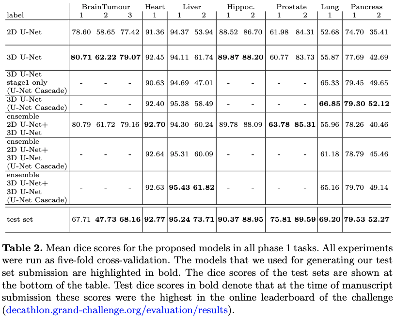
This work is built upon the original UNet (so they named it non-new UNet) and brings some automatic adaptation features instead of implementing specific architecture tweaks for a specific task. The results are the state of the art.