0. Introduction

Identifying neuronal structure in images of biological neurons captured by Transmission Electron Microscopy (ssTEM) are commonly used to perform functional analysis of the brain and other nervous systems. However, the annotation of this kind of images is very challenging, even for human experts. The ssTEM images can depict more than tens of thousands of neurons where each neuron may have thousands of synaptic connections. Consequently, the demand for automatic solutions is high and deep learning is well adapted for this type of task.

This paper proposes a solution closed to U-Net (but performs better) and is evaluated on EM segmentation challenge.

1. Related Work

Ciresan et al. (2012) [1] used a Convolutional Neural Networks (CNN) to classify pixels per pixels by using a square window centered on the considered pixel. This allowed a pixel-wise classification context-aware. This method achieved the best performance in 2012 ISBI neuronal structure segmentation challenge. Other method focused on the post-processing of the probability maps generated by a model such as Uzunbas, Chen, and Metaxsas (2014) [2], Nunez-Iglesias et al. (2013) [3] or Liu et al. (2014) [4] to improve the performance. These methods significantly outperformed Ciresan et al. (2012) [1]. However compared to human level accuracy, there is still a significant gap. The sliding window approach has actually 2 major drawbacks. The first reason is the computational cost. Considering the size of the images (order to terabytes) this solution is hardly scalable. The second point is related to the size of the window itself: the neuronal structures size can vary a lot.

2. Deep Contextual Segmentation Network Architecture

2.1. Architecture

To overcome the issue related to the sliding window's size, the authors proposed to incorporate a multi-level contextual information with different receptive fields size. They also made their architecture deeper and integrated auxiliary supervised classifiers to increase the back-propagation flow. This architecture is inspired from Long, Shelhamer, and Darrell (2014) [5] and their Fully Convolutional Networks (FCN). It contains 2 paths: downsampler or "encoder" and upsampler or "decoder". The detailed architecture is described in the figure 2.

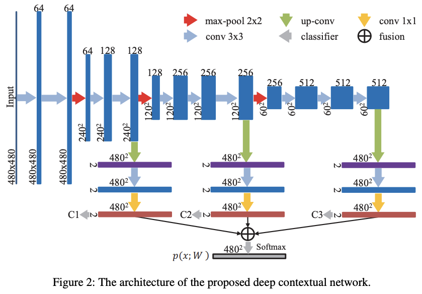
Abstract information from higher layers helps to classify while local information from low layers enables localization. At the end these multi-level contextual information are summed up together (fusion on the figure 2) and go through a softmax layer to output the probability maps.

Specifically, the architecture of neural network contains 16 convolutional layers, 3 max-pooling layers for downsampling and 3 deconvolutional layers for upsampling. The convolutional layers along with convolutional kernels (3 × 3 or 1 × 1) perform linear mapping with shared parameters. The max-pooling layers downsample the size of feature maps by the max-pooling operation (kernel size 2 × 2 with a stride 2). The deconvolutional layers upsample the size of feature maps by the backwards strided convolution.

As it is, during training occurs the problem of vanishing gradients. To overcome this issue, the authors added auxiliary classifiers C1, C2 and C3 showed in the figure 2.

2.2. Variable Receptive Field

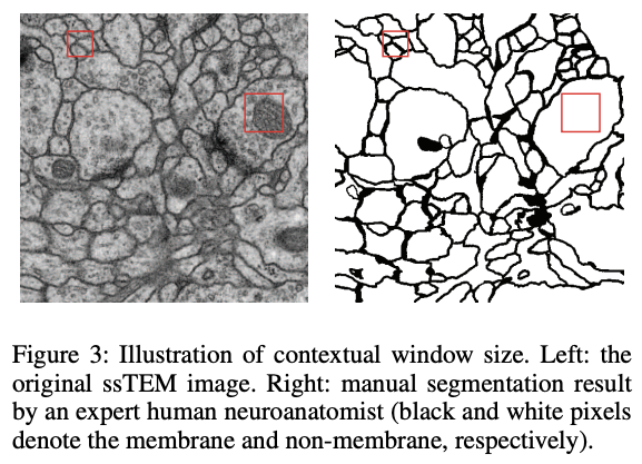
As shown in the figure 3, the area of interest can vary significantly considering the context. The architecture allows the receptive field to become larger with the increasing depth.

3. Loss Function

The classification is performed pixel-wise and the loss function is computed as:

$\mathcal{L}(\mathcal{X};\theta)= \frac{\lambda}{2}(\sum_c \parallel W_c \parallel_2^2 + \parallel W \parallel_2^2)-\sum_c \sum_{x \in \mathcal{X}}w_c \psi_c (x,\ell(x))-\sum_{x \in \mathcal{X}}\psi(x,\ell(x))$

Where the left (before the double sum) member is the regularization term and the right one the loss itself. The $\lambda$ parameter controls the tradeoff between these two terms. $W$ are the models parameters, $psi(x,\ell(x))$ the cross entropy with $\ell(x)$ the true label for a pixel $x$. Similarly $\psi_c$ is the cross entropy for the $c$th classifier (C1, C2 and C3) and $W_c$ its parameters. All parameters are jointly optimized in an end-to-end manner.

4. Post-process

The author observed that the membrane of ambiguous regions can sometimes be discontinued. For that, they are using a watershed algorithm (Beucher and Lantuejoul (1979) [6]) and the final probability map is obtained by:

$p_f(x)=w_fp(x)+(1-w_f)p_w(x)$

With $p_w(x)$ the binary contour, $p(x)$ the probability map output by the model and $w_f$ a parameter determined by obtaining the optimal result of rand error on the training data in their experiments.

5. Experiments

The models are trained on 2012 ISBSI EM Segmentation challenge and the input images are 480x480. They used a fixed learning rate decay (decreased by factor 10 every 2k iterations). The training time is about 2 hours on a Titan X.

The metrics are defined as follow:

• Rand error: 1 - the maximal F-score of the foreground-restricted rand index (Rand 1971), a measure of similarity between two clusters or segmentations. For the EM segmentation evaluation, the zero component of the original labels (background pixels of the ground truth) is excluded.
• Warping error: a segmentation metric that penalizes the topological disagreements (object splits and mergers). Pixel error: 1 - the maximal F-score of pixel similarity, or squared Euclidean distance between the original and the result labels.
• Pixel error: 1 - the maximal F-score of pixel similarity, or squared Euclidean distance between the original and the result labels.

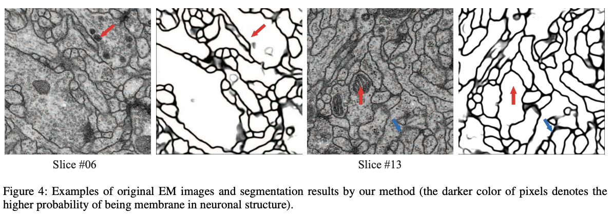
The figure 4 gives some examples of the results.

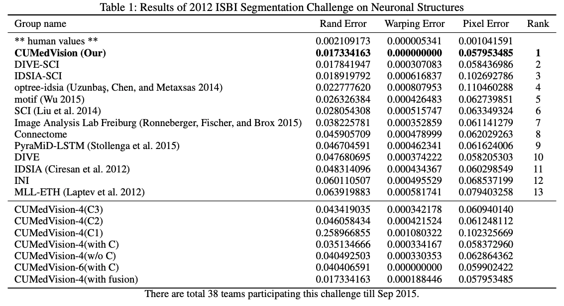
The table 1 gives the results and the ablation study. CUMedVision-6(with C) is the best model without post-processing. When adding the post-processing, CUMedVision achieve the best results. In the ablation study (lower part of the table 1), we can see that the use of the 3 auxiliary improves significantly the results. The fusion operator improve them further.

6. Conclusion

This work push further the performance increase initiated by Ciresan et al. (2012) [1] by adapting the FCN architecture. It also decrease significantly the training time (from 10 to 3 hours) compared to Ronneberger, Fischer, and Brox (2015) [7].

References

1. Ciresan, D.C., Gambardella, L.M., Giusti, A., Schmidhuber, J.: Deep neural networks segment neuronal membranes in electron microscopy images. In: NIPS. pp. 2852–2860 (2012).
2. Uzunbas¸, M. G.; Chen, C.; and Metaxsas, D. 2014. Optree: a learning-based adaptive watershed algorithm for neuron segmentation. In Medical Image Computing and ComputerAssisted Intervention MICCAI 2014. Springer. 97–105.
3. Nunez-Iglesias, J.; Kennedy, R.; Parag, T.; Shi, J.; Chklovskii, D. B.; and Zuo, X.-N. 2013. Machine learning of hierarchical clustering to segment 2d and 3d images. PloS one 8(8):08.
4. Liu, T.; Jones, C.; Seyedhosseini, M.; and Tasdizen, T. 2014. A modular hierarchical approach to 3d electron microscopy image segmentation. Journal of neuroscience methods 226:88–102.
5. Long, J.; Shelhamer, E.; and Darrell, T. 2014. Fully convolutional networks for semantic segmentation. arXiv preprint arXiv:1411.4038.
6. Beucher, S., and Lantuejoul, C. 1979. Use of watersheds in contour detection. In International Conference on Image Processing.
7. Ronneberger, O.; Fischer, P.; and Brox, T. 2015. U-net: Convolutional networks for biomedical image segmentation. arXiv preprint arXiv:1505.04597.