- Published on
Semantic Segmentation with tf.data in TensorFlow 2 and ADE20K dataset
- Authors
- Name
- Yann Le Guilly
- @yannlg_


The code is available on Google Colab: ![]()
Update 20/04/26: Fix a bug in the Google Colab version (thanks to Agapetos!) and add a few external links.
Update 20/04/25: Update the whole article to be easier to run the code. Also, add a link to run it on Google Colab.
1. Introduction
In this notebook we are going to cover the usage of TensorFlow 2 and tf.data on a popular semantic segmentation 2D images dataset: ADE20K.
The type of data we are going to manipulate consists in:
- a jpg image with 3 channels (RGB)
- a jpg mask with 1 channel (for each pixel we have 1 true class over 150 possible)
You can also find all the information by reading the official TensorFlow tutorials:
- https://www.tensorflow.org/tutorials/load_data/images
- https://www.tensorflow.org/tutorials/images/segmentation
This notebook assumes that you already downloaded ADE20k and extracted the content of the archive in ./data/ADEChallengeData2016/ with ./ meaning the directory where this notebook is running.
You can download it here: http://sceneparsing.csail.mit.edu/
Also, if you run this notebook, a GPU is almost mandatory since the computations take A LOT of time on CPU.
2. Preparing the Environment
from glob import glob

import IPython.display as display
import matplotlib.pyplot as plt
import numpy as np
import tensorflow as tf
import datetime, os
from tensorflow.keras.layers import *
from tensorflow.keras.callbacks import EarlyStopping, ModelCheckpoint
from tensorflow.keras.optimizers import Adam
from IPython.display import clear_output
import tensorflow_addons as tfa

# For more information about autotune:
# https://www.tensorflow.org/guide/data_performance#prefetching
AUTOTUNE = tf.data.experimental.AUTOTUNE
print(f"Tensorflow ver. {tf.__version__}")
Tensorflow ver. 2.1.0
# important for reproducibility
# this allows generating the same random numbers
SEED = 42
# you can change this path to reflect your own settings if necessary
dataset_path = "data/ADEChallengeData2016/images/"
training_data = "training/"
val_data = "validation/"
By default, TensorFlow uses 100% of the available GPU memory. It allows to do contiguous memory allocation with is potentially faster. You can deactivate this default behavior. I feel useful the fact that I can check how much memory is used considering the batch size.
gpus = tf.config.experimental.list_physical_devices('GPU')
if gpus:
    try:
        for gpu in gpus:
            tf.config.experimental.set_memory_growth(gpu, True)
        logical_gpus = tf.config.experimental.list_logical_devices('GPU')
        print(len(gpus), "Physical GPUs,", len(logical_gpus), "Logical GPUs")
    except RuntimeError as e:
        print(e)
1 Physical GPU, 1 Logical GPU
3. Creating our Dataloader
# Image size that we are going to use
IMG_SIZE = 128
# Our images are RGB (3 channels)
N_CHANNELS = 3
# Scene Parsing has 150 classes + `not labeled`
N_CLASSES = 151
3.1. Creating a source dataset
TRAINSET_SIZE = len(glob(dataset_path + training_data + "*.jpg"))
print(f"The Training Dataset contains {TRAINSET_SIZE} images.")

VALSET_SIZE = len(glob(dataset_path + val_data + "*.jpg"))
print(f"The Validation Dataset contains {VALSET_SIZE} images.")
The Training Dataset contains 20210 images. The Validation Dataset contains 2000 images.
For each image of our dataset, we will apply some operations wrapped into a function. Then we will map the whole dataset with this function.
So let's write this function:
def parse_image(img_path: str) -> dict:
    """Load an image and its annotation (mask) and returning
    a dictionary.

    Parameters
    ----------
    img_path : str
        Image (not the mask) location.

    Returns
    -------
    dict
        Dictionary mapping an image and its annotation.
    """
    image = tf.io.read_file(img_path)
    image = tf.image.decode_jpeg(image, channels=3)
    image = tf.image.convert_image_dtype(image, tf.uint8)

    # For one Image path:
    # .../trainset/images/training/ADE_train_00000001.jpg
    # Its corresponding annotation path is:
    # .../trainset/annotations/training/ADE_train_00000001.png
    mask_path = tf.strings.regex_replace(img_path, "images", "annotations")
    mask_path = tf.strings.regex_replace(mask_path, "jpg", "png")
    mask = tf.io.read_file(mask_path)
    # The masks contain a class index for each pixels
    mask = tf.image.decode_png(mask, channels=1)
    # In scene parsing, "not labeled" = 255
    # But it will mess up with our N_CLASS = 150
    # Since 255 means the 255th class
    # Which doesn't exist
    mask = tf.where(mask == 255, np.dtype('uint8').type(0), mask)
    # Note that we have to convert the new value (0)
    # With the same dtype than the tensor itself

    return {'image': image, 'segmentation_mask': mask}
In case you would like to load any other image format, you should modify the parse_image function. TensorFlow I/O provides additional tools that might help you. For example, in the case of loading TIFF images, you can use:
import tensorflow as tf
import tensorflow.io as tfio
...
def parse_image(img_path: str) -> dict:
...
image = tf.io.read_file(img_path)
tfio.experimental.image.decode_tiff(image)
...
In this case, don't forget to modify the number of channels when implementing the model later.
train_dataset = tf.data.Dataset.list_files(dataset_path + training_data + "*.jpg", seed=SEED)
train_dataset = train_dataset.map(parse_image)

val_dataset = tf.data.Dataset.list_files(dataset_path + val_data + "*.jpg", seed=SEED)
val_dataset =val_dataset.map(parse_image)
3.2. Applying some transformations to our dataset
# Here we are using the decorator @tf.function
# if you want to know more about it:
# https://www.tensorflow.org/api_docs/python/tf/function

@tf.function
def normalize(input_image: tf.Tensor, input_mask: tf.Tensor) -> tuple:
    """Rescale the pixel values of the images between 0.0 and 1.0
    compared to [0,255] originally.

    Parameters
    ----------
    input_image : tf.Tensor
        Tensorflow tensor containing an image of size [SIZE,SIZE,3].
    input_mask : tf.Tensor
        Tensorflow tensor containing an annotation of size [SIZE,SIZE,1].

    Returns
    -------
    tuple
        Normalized image and its annotation.
    """
    input_image = tf.cast(input_image, tf.float32) / 255.0
    return input_image, input_mask

@tf.function
def load_image_train(datapoint: dict) -> tuple:
    """Apply some transformations to an input dictionary
    containing a train image and its annotation.

    Notes
    -----
    An annotation is a regular channel image.
    If a transformation such as rotation is applied to the image,
    the same transformation has to be applied to the annotation also.

    Parameters
    ----------
    datapoint : dict
        A dict containing an image and its annotation.

    Returns
    -------
    tuple
        A modified image and its annotation.
    """
    input_image = tf.image.resize(datapoint['image'], (IMG_SIZE, IMG_SIZE))
    input_mask = tf.image.resize(datapoint['segmentation_mask'], (IMG_SIZE, IMG_SIZE))

    if tf.random.uniform(()) > 0.5:
        input_image = tf.image.flip_left_right(input_image)
        input_mask = tf.image.flip_left_right(input_mask)

    input_image, input_mask = normalize(input_image, input_mask)

    return input_image, input_mask

@tf.function
def load_image_test(datapoint: dict) -> tuple:
    """Normalize and resize a test image and its annotation.

    Notes
    -----
    Since this is for the test set, we don't need to apply
    any data augmentation technique.

    Parameters
    ----------
    datapoint : dict
        A dict containing an image and its annotation.

    Returns
    -------
    tuple
        A modified image and its annotation.
    """
    input_image = tf.image.resize(datapoint['image'], (IMG_SIZE, IMG_SIZE))
    input_mask = tf.image.resize(datapoint['segmentation_mask'], (IMG_SIZE, IMG_SIZE))

    input_image, input_mask = normalize(input_image, input_mask)

    return input_image, input_mask
Manipulating datasets in tensorflow can be complicated. You can read the official documentation to understand how they are working: https://www.tensorflow.org/guide/data#training_workflows
BATCH_SIZE = 32

# for reference about the BUFFER_SIZE in shuffle:
# https://stackoverflow.com/questions/46444018/meaning-of-buffer-size-in-dataset-map-dataset-prefetch-and-dataset-shuffle
BUFFER_SIZE = 1000

dataset = {"train": train_dataset, "val": val_dataset}

# -- Train Dataset --#
dataset['train'] = dataset['train'].map(load_image_train, num_parallel_calls=tf.data.experimental.AUTOTUNE)
dataset['train'] = dataset['train'].shuffle(buffer_size=BUFFER_SIZE, seed=SEED)
dataset['train'] = dataset['train'].repeat()
dataset['train'] = dataset['train'].batch(BATCH_SIZE)
dataset['train'] = dataset['train'].prefetch(buffer_size=AUTOTUNE)

#-- Validation Dataset --#
dataset['val'] = dataset['val'].map(load_image_test)
dataset['val'] = dataset['val'].repeat()
dataset['val'] = dataset['val'].batch(BATCH_SIZE)
dataset['val'] = dataset['val'].prefetch(buffer_size=AUTOTUNE)

print(dataset['train'])
print(dataset['val'])

# how shuffle works: https://stackoverflow.com/a/53517848

<PrefetchDataset shapes: ((None, 128, 128, 3), (None, 128, 128, 1)), types: (tf.float32, tf.float32)>
<PrefetchDataset shapes: ((None, 128, 128, 3), (None, 128, 128, 1)), types: (tf.float32, tf.float32)>
4. Visualizing the Dataset
It seems everything is fine. It can be very hard to build your model by having bugs in your dataset. This makes the development process very painful since the potential bugs from your model are adding up to the potential bugs in your dataloaders. Therefore, it is recommended to make sure that you have what you expect.
For that, we are going to develop simple functions to visualize the content of our dataloaders.
def display_sample(display_list):
    """Show side-by-side an input image,
    the ground truth and the prediction.
    """
    plt.figure(figsize=(18, 18))

    title = ['Input Image', 'True Mask', 'Predicted Mask']

    for i in range(len(display_list)):
        plt.subplot(1, len(display_list), i+1)
        plt.title(title[i])
        plt.imshow(tf.keras.preprocessing.image.array_to_img(display_list[i]))
        plt.axis('off')
    plt.show()
for image, mask in dataset['train'].take(1):
    sample_image, sample_mask = image, mask

display_sample([sample_image[0], sample_mask[0]])


The dimensions are the ones we expect and it shows up properly. We can start the development of the model itself.
5. Developing the Model (UNet) Using Keras Functional API
For this example, we are going to implement a popular architecture: UNet. In a sense, it is not the best for a tutorial since this model is very heavy. But I found the exercise interesting. Especially because we are going to use the functional API provided by Keras.
This architecture was introduced in the paper U-Net: Convolutional Networks for Biomedical Image Segmentation that you can read here: https://arxiv.org/abs/1505.04597
You can also read my notes on this paper here: https://yann-leguilly.gitlab.io/post/2019-12-11-unet-biomedical-images/
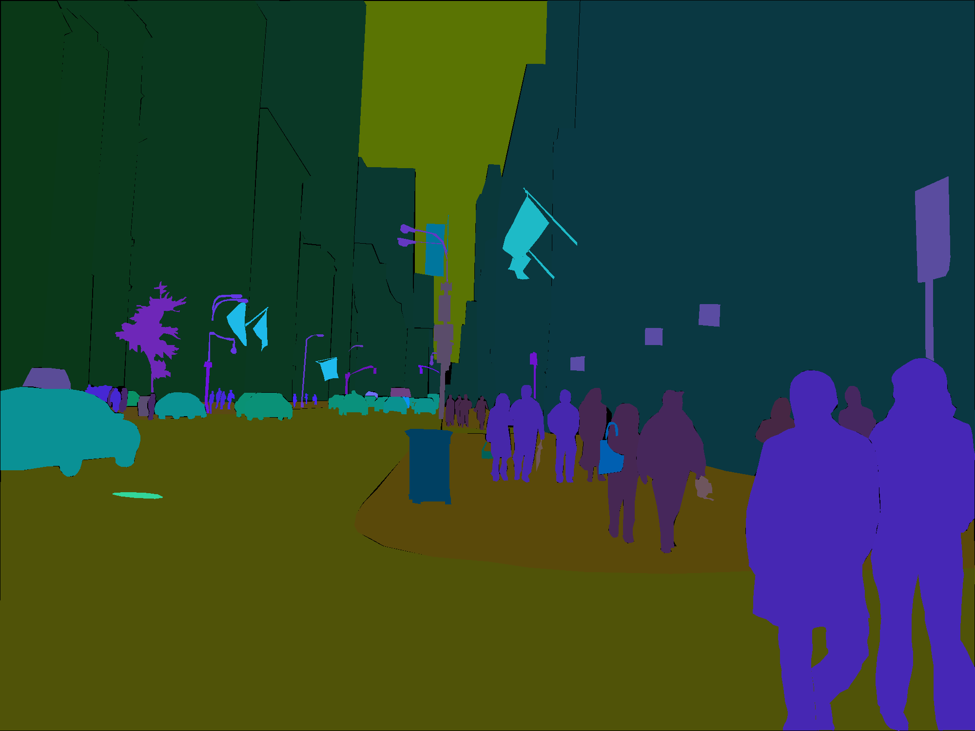
We are going to reproduce this:


5.1. Implementation
# -- Keras Functional API -- #
# -- UNet Implementation -- #
# Everything here is from tensorflow.keras.layers
# I imported tensorflow.keras.layers * to make it easier to read
dropout_rate = 0.5
input_size = (IMG_SIZE, IMG_SIZE, N_CHANNELS)

# If you want to know more about why we are using `he_normal`:
# https://stats.stackexchange.com/questions/319323/whats-the-difference-between-variance-scaling-initializer-and-xavier-initialize/319849#319849
# Or the excellent fastai course:
# https://github.com/fastai/course-v3/blob/master/nbs/dl2/02b_initializing.ipynb
initializer = 'he_normal'


# -- Encoder -- #
# Block encoder 1
inputs = Input(shape=input_size)
conv_enc_1 = Conv2D(64, 3, activation='relu', padding='same', kernel_initializer=initializer)(inputs)
conv_enc_1 = Conv2D(64, 3, activation = 'relu', padding='same', kernel_initializer=initializer)(conv_enc_1)

# Block encoder 2
max_pool_enc_2 = MaxPooling2D(pool_size=(2, 2))(conv_enc_1)
conv_enc_2 = Conv2D(128, 3, activation = 'relu', padding = 'same', kernel_initializer = initializer)(max_pool_enc_2)
conv_enc_2 = Conv2D(128, 3, activation = 'relu', padding = 'same', kernel_initializer = initializer)(conv_enc_2)

# Block  encoder 3
max_pool_enc_3 = MaxPooling2D(pool_size=(2, 2))(conv_enc_2)
conv_enc_3 = Conv2D(256, 3, activation = 'relu', padding = 'same', kernel_initializer = initializer)(max_pool_enc_3)
conv_enc_3 = Conv2D(256, 3, activation = 'relu', padding = 'same', kernel_initializer = initializer)(conv_enc_3)

# Block  encoder 4
max_pool_enc_4 = MaxPooling2D(pool_size=(2, 2))(conv_enc_3)
conv_enc_4 = Conv2D(512, 3, activation = 'relu', padding = 'same', kernel_initializer = initializer)(max_pool_enc_4)
conv_enc_4 = Conv2D(512, 3, activation = 'relu', padding = 'same', kernel_initializer = initializer)(conv_enc_4)
# -- Encoder -- #

# ----------- #
maxpool = MaxPooling2D(pool_size=(2, 2))(conv_enc_4)
conv = Conv2D(1024, 3, activation = 'relu', padding = 'same', kernel_initializer = initializer)(maxpool)
conv = Conv2D(1024, 3, activation = 'relu', padding = 'same', kernel_initializer = initializer)(conv)
# ----------- #

# -- Decoder -- #
# Block decoder 1
up_dec_1 = Conv2D(512, 2, activation = 'relu', padding = 'same', kernel_initializer = initializer)(UpSampling2D(size = (2,2))(conv))
merge_dec_1 = concatenate([conv_enc_4, up_dec_1], axis = 3)
conv_dec_1 = Conv2D(512, 3, activation = 'relu', padding = 'same', kernel_initializer = initializer)(merge_dec_1)
conv_dec_1 = Conv2D(512, 3, activation = 'relu', padding = 'same', kernel_initializer = initializer)(conv_dec_1)

# Block decoder 2
up_dec_2 = Conv2D(256, 2, activation = 'relu', padding = 'same', kernel_initializer = initializer)(UpSampling2D(size = (2,2))(conv_dec_1))
merge_dec_2 = concatenate([conv_enc_3, up_dec_2], axis = 3)
conv_dec_2 = Conv2D(256, 3, activation = 'relu', padding = 'same', kernel_initializer = initializer)(merge_dec_2)
conv_dec_2 = Conv2D(256, 3, activation = 'relu', padding = 'same', kernel_initializer = initializer)(conv_dec_2)

# Block decoder 3
up_dec_3 = Conv2D(128, 2, activation = 'relu', padding = 'same', kernel_initializer = initializer)(UpSampling2D(size = (2,2))(conv_dec_2))
merge_dec_3 = concatenate([conv_enc_2, up_dec_3], axis = 3)
conv_dec_3 = Conv2D(128, 3, activation = 'relu', padding = 'same', kernel_initializer = initializer)(merge_dec_3)
conv_dec_3 = Conv2D(128, 3, activation = 'relu', padding = 'same', kernel_initializer = initializer)(conv_dec_3)

# Block decoder 4
up_dec_4 = Conv2D(64, 2, activation = 'relu', padding = 'same', kernel_initializer = initializer)(UpSampling2D(size = (2,2))(conv_dec_3))
merge_dec_4 = concatenate([conv_enc_1, up_dec_4], axis = 3)
conv_dec_4 = Conv2D(64, 3, activation = 'relu', padding = 'same', kernel_initializer = initializer)(merge_dec_4)
conv_dec_4 = Conv2D(64, 3, activation = 'relu', padding = 'same', kernel_initializer = initializer)(conv_dec_4)
conv_dec_4 = Conv2D(2, 3, activation = 'relu', padding = 'same', kernel_initializer = initializer)(conv_dec_4)
# -- Dencoder -- #

output = Conv2D(N_CLASSES, 1, activation = 'softmax')(conv_dec_4)
Now we can load and compile the model to make sure that there are no bugs.
model = tf.keras.Model(inputs = inputs, outputs = output)
model.compile(optimizer=Adam(learning_rate=0.0001), loss = tf.keras.losses.SparseCategoricalCrossentropy(),
              metrics=['accuracy'])
5.2. Sanity Check
We can visualize a sample prediction to be sure that we see what we expect.
def create_mask(pred_mask: tf.Tensor) -> tf.Tensor:
    """Return a filter mask with the top 1 predictions
    only.

    Parameters
    ----------
    pred_mask : tf.Tensor
        A [IMG_SIZE, IMG_SIZE, N_CLASS] tensor. For each pixel we have
        N_CLASS values (vector) representing the probability of the pixel being these classes. Example: A pixel with the vector [0.0, 0.0, 1.0]
        has been predicted class 2 with a probability of 100%.

    Returns
    -------
    tf.Tensor
        A [IMG_SIZE, IMG_SIZE, 1] mask with top 1 predictions
        for each pixels.
    """
    # pred_mask -> [IMG_SIZE, SIZE, N_CLASS]
    # 1 prediction for each class but we want the highest score only
    # so we use argmax
    pred_mask = tf.argmax(pred_mask, axis=-1)
    # pred_mask becomes [IMG_SIZE, IMG_SIZE]
    # but matplotlib needs [IMG_SIZE, IMG_SIZE, 1]
    pred_mask = tf.expand_dims(pred_mask, axis=-1)
    return pred_mask

def show_predictions(dataset=None, num=1):
    """Show a sample prediction.

    Parameters
    ----------
    dataset : [type], optional
        [Input dataset, by default None
    num : int, optional
        Number of sample to show, by default 1
    """
    if dataset:
        for image, mask in dataset.take(num):
            pred_mask = model.predict(image)
            display_sample([image[0], true_mask, create_mask(pred_mask)])
    else:
        # The model is expecting a tensor of the size
        # [BATCH_SIZE, IMG_SIZE, IMG_SIZE, 3]
        # but sample_image[0] is [IMG_SIZE, IMG_SIZE, 3]
        # and we want only 1 inference to be faster
        # so we add an additional dimension [1, IMG_SIZE, IMG_SIZE, 3]
        one_img_batch = sample_image[0][tf.newaxis, ...]
        # one_img_batch -> [1, IMG_SIZE, IMG_SIZE, 3]
        inference = model.predict(one_img_batch)
        # inference -> [1, IMG_SIZE, IMG_SIZE, N_CLASS]
        pred_mask = create_mask(inference)
        # pred_mask -> [1, IMG_SIZE, IMG_SIZE, 1]
        display_sample([sample_image[0], sample_mask[0],
                        pred_mask[0]])
for image, mask in dataset['train'].take(1):
    sample_image, sample_mask = image, mask

show_predictions()
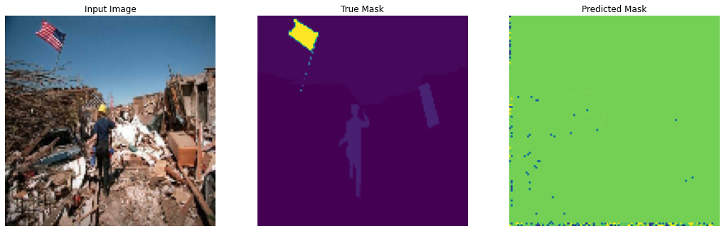
The far-right image is a prediction with random weights. We are ready to start the training!
6. Training our Model
6.1. Simpler training loop
Let's run a simple training loop with only 1 epoch first.
EPOCHS = 1

STEPS_PER_EPOCH = TRAINSET_SIZE // BATCH_SIZE
VALIDATION_STEPS = VALSET_SIZE // BATCH_SIZE
# sometimes it can be very interesting to run some batches on CPU
# because the tracing is way better than on GPU
# you will have a more obvious error message
# but in our case, it takes A LOT of time

# On CPU
# with tf.device("/cpu:0"):
#     model_history = model.fit(dataset['train'], epochs=EPOCHS,
#                               steps_per_epoch=STEPS_PER_EPOCH,
#                               validation_steps=VALIDATION_STEPS,
#                               validation_data=dataset['val'])

# On GPU
model_history = model.fit(dataset['train'], epochs=EPOCHS,
                          steps_per_epoch=STEPS_PER_EPOCH,
                          validation_steps=VALIDATION_STEPS,
                          validation_data=dataset['val'])
Train for 631 steps, validate for 62 steps
631/631 [==============================]
- 184s 292ms/step
- loss: 4.5188
- accuracy: 0.0957
- val_loss: 3.9329
- val_accuracy: 0.1289
Everything looks great! We can start our 'real' training.
6.2. More Advanced Training Loop
Keras implements what we call 'callbacks'. We can use them to run custom functions at any step of the training. Here we are going to show the output of the model compared to the original image and the ground truth after each epoch. We are also going to collect some useful metrics to make sure our training is happening well by using tensorboard.
class DisplayCallback(tf.keras.callbacks.Callback):
    def on_epoch_end(self, epoch, logs=None):
        clear_output(wait=True)
        show_predictions()
        print ('\nSample Prediction after epoch {}\n'.format(epoch+1))
EPOCHS = 5

logdir = os.path.join("logs", datetime.datetime.now().strftime("%Y%m%d-%H%M%S"))
tensorboard_callback = tf.keras.callbacks.TensorBoard(logdir, histogram_freq=1)

callbacks = [
    # to show samples after each epoch
    DisplayCallback(),
    # to collect some useful metrics and visualize them in tensorboard
    tensorboard_callback,
    # if no accuracy improvements we can stop the training directly
    tf.keras.callbacks.EarlyStopping(patience=10, verbose=1),
    # to save checkpoints
    tf.keras.callbacks.ModelCheckpoint('best_model_unet.h5', verbose=1, save_best_only=True, save_weights_only=True)
]

model = tf.keras.Model(inputs = inputs, outputs = output)

# here I'm using a new optimizer: https://arxiv.org/abs/1908.03265
optimizer=tfa.optimizers.RectifiedAdam(lr=1e-3)

loss = tf.keras.losses.SparseCategoricalCrossentropy()
model.compile(optimizer=optimizer, loss = loss,
                  metrics=['accuracy'])
model = train_model(model, optimizer, loss, callbacks)
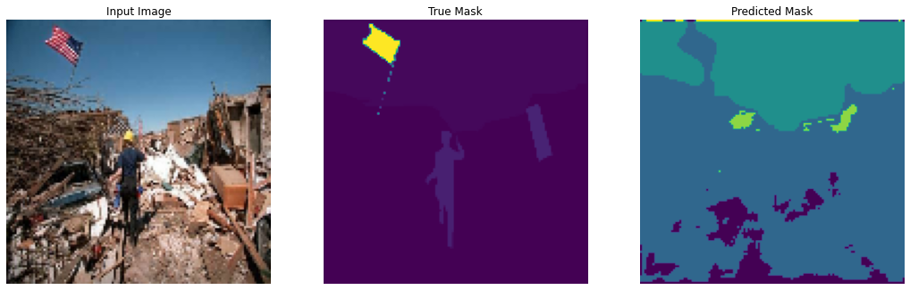
Sample Prediction after epoch 5
Epoch 00005: val_loss improved from 2.76228 to 2.71097, saving model to best_model_unet.h5
631/631 [==============================]
- 189s 299ms/step
- loss: 2.7291
- accuracy: 0.3685
- val_loss: 2.7110
- val_accuracy: 0.3773
6.3. Monitoring the training
While your model is training, you want to monitor some metrics. To do this, tensorboard is a common tool (I will write another article about this topic later). I also feel useful to monitor your GPU(s)/CPU(s).


I'm usually using nvtop to monitor my GPU and htop for the CPU.
7. Conclusion
This was a simple example of how to
- load a specific dataset
- implement your model (UNet)
- Simple training loop using
model.fit()
The code is available on Google Colab:![]()
and Github: https://github.com/dhassault/tf-semantic-example