You can find the paper here: https://arxiv.org/abs/1505.04597.

0. Introduction

The goal of this work is to learn to localize precisely specific patterns. This need comes from the biomedical field where it is difficult to collect a large amount of (annotated) data. There are various reasons for that and we can mention privacy or the need for an expert to annotate the data. The annotation process cannot be scaled.

The proposed architecture consists of a contracting path or "encoder" that captures the "context". This encoder is followed by an expanding path or "decoder" and enables the precise localization of patterns.

On the task itself, biomedical image processing has also specific constraints. Unlike a simple classification by conventional Convolutional Neural Networks (CNN), pixel-wise classification is often required. This type of task is called Segmentation (it includes Instance, Semantic and Panoptic Segmentation). Also as we mentioned earlier, the number of data is very limited.

1. Related Work

Ciresan et al. [1] proposed a sliding-window architecture that can localize and is less data-eager. But this network is slow and there is a lot of redundancy in the computations. Also due to the architecture itself, a trade-off has to be set between localization accuracy and the use of context. Seyedhosseini et al. [2] and Hariharan et al. [3] introduce a multilayer architecture that could perform good localization and the use of the context at the same time. This work is built upon a Fully Convolutional Architecture (FCN) proposed by Long et al. [4].

2. U-Net Architecture

The main idea introduced by Long et al. [4] is to increase the output resolution of the architecture by using upsampling operators instead of pooling. To localize, high-resolution features from the encoder are combined with the upsampled output. It allows the models to assemble a more precise mask.

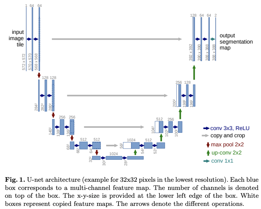
One important contribution of this work is the addition of a large number of feature channels in the upsampling operations. This allows the network to propagate more contextual information to higher resolution layers. This implies that the decoder is roughly symmetric to the encoder since the "contextual embeddings" are propagated from one path to the other. This yields to the u-shaped architecture given in figure 1.

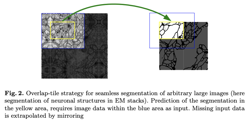
As opposed to the FNC architecture, U-Net has no fully connected layers. The segmentation map contains only the pixels for which the full context is available in the input image. An overlap-tile strategy is used to segment arbitrarily images and the missing input data is extrapolated by using padding of the input image (padding 'same' in PyTorch). An example is given in figure 2.

Overall the encoder consists of repeated 2 3x3 convolutions (unpadded), followed by a ReLU and a 2x2 max pooling with stride 2 for downsampling. In the next group of layers (still in the encoder), the number of feature channels is doubled (64 → 128 → 256 → 512 in figure 1).

The decoder path is a series of upsampling operations of the feature map followed by a 2x2 convolution that halves the number of features channels. We can find here the symmetry. Each step is concatenated with the corresponding feature map from the decoder. The feature maps are cropped since the border is lost because of the convolutions (see CS231n). Finally, the groups of layers (step) are followed by two 3x3 convolutions and a ReLU.

3. Datasets & Data Augmentation

The model is crafted to perform specifically on ISBI (includes 2 datasets) and EM segmentation challenges. These datasets consist of segmenting cells. This task is called instance segmentation. This brings its challenges. For example, the cells are very close to each other. And to segment them properly, the model has to learn the separation in-between cells. This problem is addressed and will be described in the next part. Another specific aspect is that the invariance of the shape of the cells can be simulated easily. This is done in the data augmentation. The authors noted that random elastic deformations are a key concept for training a segmentation model with very few training images.

The elastic data augmentation is a displacement sampled from a Gaussian distribution with 10 pixels std. The displacement is then computed by using a bicubic interpolation. This is done by using morphological operations:

4. Loss Function

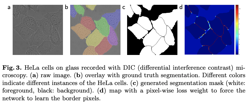
Adding to the data augmentation, a few training tricks are also applied to overcome the challenges related to this particular dataset. A first weight map is pre-computed to give a higher weight on the pixels that belong to cells instead of the background. This is shown in figure 3c. The result is a weight map $w_c(x)$. Then, based on the ground truth (figure 3b) the authors also assign a higher weight to the thin borders that separate cells (figure 3d). The final weight map is obtained by:

where $w_c : \Omega \rightarrow \R$ is the weight map that emphasize the cells pixels over the background, $d_1: \Omega \rightarrow \R$ is the distance to the border of the nearest cell, $d_2: \Omega \rightarrow \R$. Finally $w_0=10$ and $\sigma \approx 5$ are parameters set by the authors. No further information are given regarding their value.

A soft-max function is also applied pixel-wise on the final feature map:

where $a_k(x)$ is the activation feature channel $k$ at the pixel position $x \in \Omega$ with $\Omega \subset \Z^2$. $K$ is the number of classes and $pk(x)$ is the approximated maximum-function. For $p_k \approx 1$ for $k$ with the maximum activation otherwise $p_k \approx 0$.

The weight map and the soft-max are then combined in the loss function:

5. Experiments

As mentioned earlier, one dataset is the EM segmentation challenge. It consists of 30 images of 512x512 pixels. As always in challenges, the test set provided without ground truth. The results are given in Table 1.

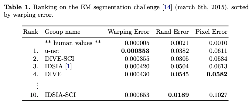
The metrics details are given in [5]. The wrapping error is significantly better than the architecture proposed by Ciresan et al. [1] as for the rand error. Regarding the rand error, IDSIA-SCI is performing better than U-Net. But this model uses a highly specific dataset to post-process the output probability map. For U-Net, no post-processing is applied.

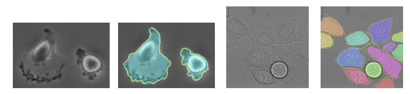
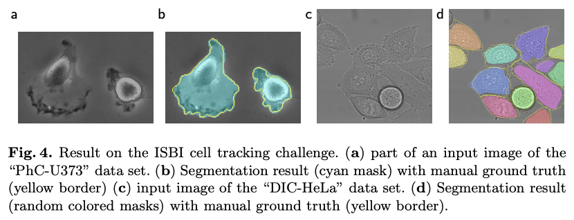
The next set of datasets are "PhC-U373" and "DIC-HeLa". Some examples are given in figure 4.

The results on these datasets are given in table 2.

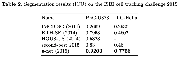
U-Net outperforms significantly all previous architecture with an IoU of 0.9203 on PhC-U373 and 0.7756 on DIC-HeLa. Especially on the latter since the previous results are IoU 0.46 (as opposed to 0.7756 for U-Net).

6. Conclusion

U-Net is a great improvement compared to previous state-of-the-art and without any post-processing. It is also customized for the very specific characteristics of biomedical image processing.

References

1. Ciresan, D.C., Gambardella, L.M., Giusti, A., Schmidhuber, J.: Deep neural networks segment neuronal membranes in electron microscopy images. In: NIPS. pp. 2852–2860 (2012)
2. Seyedhosseini, M., Sajjadi, M., Tasdizen, T.: Image segmentation with cascaded hierarchical models and logistic disjunctive normal networks. In: Computer Vision (ICCV), 2013 IEEE International Conference on. pp. 2168–2175 (2013)
3. Hariharan, B., Arbelez, P., Girshick, R., Malik, J.: Hypercolumns for object segmentation and fine-grained localization (2014), arXiv:1411.5752 [cs.CV]
4. Long, J., Shelhamer, E., Darrell, T.: Fully convolutional networks for semantic segmentation (2014), arXiv:1411.4038 [cs.CV]
5. EM segmentation challenge, http://brainiac2.mit.edu/ isbi_challenge/