EfficientNet: Rethinking Model Scaling for Convolutional Neural Networks (May 2019)

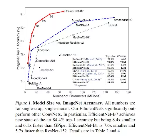
This paper was published by Mingxing Tan and Quoc V. Le, members of Google Research, Brain Team. They propose a method to scale up neural nets. Their biggest model achieves 84.4% top-1 / 97.1% top-5 accuracy on ImageNet and the state-of-the-art on CIFAR-100, while being 8.4x smaller and 6.1x faster on inference than the best existing ConvNet. The paper is available here: https://arxiv.org/abs/1905.11946.

1. Introduction

In this paper, "scaling up" is used for "increasing the accuracy of the model" in general. This includes increasing the number of layers (the depth of the model), increasing the size of the input images (resolution). This work focuses on Convolutional Neural Networks (ConvNets) and studies the particular process of scaling those architectures. Is there a principled method to scale up ConvNets that can achieve better accuracy and efficiency?

It seems that when it comes to scaling up, the best way is to increase all the dimensions width/depth/resolution by applying to them a constant ratio.

Their process is very simple. If we want to use $2^N$ , just increase the depth of the network by $\alpha^N$ , the width of the channels by $\beta^N$ and the image size by $\gamma^N$ . This is illustrated in figure 2.

The intuition of this is supported by theoretical (Raghu et al., 2017; Lu et al., 2018) and empirical results (Zagoruyko & Komodakis, 2016). Figure 1 sums up the performance increase for the number of parameters.

ConvNet Accuracy: the authors discuss how researchers improved the accuracy of models since ImageNet in 2012. But we already reached the hardware memory limit. So now we have to think about efficiency instead of increasing the number of parameters.

ConvNet Efficiency: neural architecture search (NAS) is becoming very popular and very successful when it is about finding the right trade-off between accuracy and efficiency (Waymo communicated interesting things about this). But this applies mainly to small architecture like MobileNets, ShuffleNets, and SqueezeNets. In this paper, they are exploring model efficiency for super large ConvNets.

Model Scaling: previous works showed that depth and width are both important for ConvNets' expressive power. But we don't understand how to scale them properly to achieve better efficiency (in terms of computational power) and accuracy.

3. Compound Model Scaling

3.1. Problem Formulation

A ConvNet $i$ can be defined as: $Y_i = \mathcal{F}_i(X_i)$ . The shape of the tensor $X_i$ is $\langle H_i,W_i,C_i \rangle$ . $H_i$ and $W_i$ is the resolution of the input images and

$C_i$ is the number of channels (cf. figure 2). The whole neural net is therefore defined by $\mathcal{N} = \mathcal{F}\_1 \bigodot \ldots \bigodot \mathcal{F}\_k = \bigodot\_{j=1, \ldots ,k} \mathcal{F}\_j (X)$ . Also, since the ConvNet layers have same architectures across stages, we can re-write it as:

\mathcal{N} = \bigodot\_{i=1, \ldots ,s} \mathcal{F}\_i^{L\_i} (X\_{\langle H\_i, W\_i, C\_i \rangle})

With $\bigodot$ is the Hadamard product.

Unlike finding the best architecture for the layers, this work focuses on scaling only. It simplifies the problem. Also, to further reduce the design space, they consider scaling uniformly all the architecture with a constant ratio. They formulate this problem as an optimization one:

\max_{d,w,r} Accuracy(\mathcal{N}(d,w,r))

s.t. \quad \mathcal{N}(d,w,r) = \bigodot_{i=1, \ldots,s} \hat{\mathcal{F}}_i^{d \cdot \mathcal{L}_i}(X_{\langle r \cdot \hat H_{i},r \cdot \hat W_i,w \cdot \hat C_i \rangle}

Memory(\mathcal{N}) \leq target\_memory

FLOPS(\mathcal{\mathcal{N}}) \leq target\_flops

With $w, d, r$ as the coefficients for scaling the network width, depth, and resolution of the input images. $\hat F_i, \hat L_i, \hat H_i, \hat W_i, \hat C_i$ are predefined parameters. An example of those predefined parameters is shown later in Table 1.

3.2. Scaling Dimensions

Regular methods are scaling only 1 dimension (among $w,d,r$ ).

Depth (d): most common way. But there is not so much value to increase again and again: ResNet-1000 has the same accuracy as ResNet-101.

Width (w): commonly used for small models. "... wider networks tend to be able to capture more fine-grained features and are easier to train". But "...the accuracy quickly saturates when networks become much wider than larger...".

Resolution ( r): Intuitively, higher resolution expose more details that the model can capture. But the accuracy gain is decreasing with high resolution.

3.3. Compound Scaling

Intuitively, the dimensions are not independent: if we increase the resolution of the input images, we should increase the depth of the network to be able to capture more details. This is illustrated in figure 4.

The authors propose a method that they call the compound scaling method.

depth: $d = \alpha^{\phi}$

width: $w = \beta^{\phi}$

resolution: $r = \gamma^{\phi}$

with $\alpha, \beta, \gamma$ determined by a grid search.

4. EfficientNet Architecture

The authors used both common architecture and their own to do their experimentation. Their architecture is obtained by NAS. This produced EfficientNet-B0. They targeted an architecture FLOPS optimized (means the target is the computational power efficiency). The details are given in table 1.

The main block is a mobile inverted bottleneck. Their method is done in 2 steps:

STEP 1: they first fix $\phi = 1$ , assuming twice more re-sources available, and do a small grid search of $\alpha, \beta, \gamma$ based on the optimization problem given earlier. In particular, we find the best values for EfficientNet-B0 are $\alpha = 1.2,\beta=1.1,\gamma= 1.15$ , under the constraint of $\alpha \cdot \beta^2 \cdot \gamma^2 \backsimeq 2$ .
STEP 2: they then fix $\alpha, \beta, \gamma$ as constants and scale up the baseline network with different $\phi$ , to obtain EfficientNet-B1 to B7 (details in Table 2).

5. Experiments

5.1 Scaling Up MobileNets and ResNets

First, they evaluate their method on MobileNets and ResNet. The results are given in Table 3.

5.2 ImageNet Results for EfficientNet

The training parameters are: RMSProp for the optimizer, decay 0.9, momentum 0.9, batch norm momentum 0.99, weight decay 1.e-5, learning rate 0.256 with 0.97 decay every 2.4 epochs. They also used Swish Activation (similar to ReLU), fixed AutoAugment policy, stochastic depth, and drop connect ratio of 0.3. Adding to that, they linearly increased the dropout ratio from 0.2 for EfficientNet-B0 to 0.5 for EfficientNet-B7. Table 2 shows the performance of all models. Figures 1 and 5 illustrate the parameters-accuracy and FLOPS-accuracy curves.

Table 4 shows the latency on CPU (they did 20 runs).

5.3. Transfer Learning Results for EfficientNet

In table 5, they evaluated the accuracy using transfer learning. State-of-the-art on 5 datasets on the 8 evaluated (when the paper was published...). And 9.6x fewer parameters on average.

In figure 6, they compare the accuracy-parameters curve for different models. Same as before, EfficientNets are achieving a better accuracy with fewer parameters.

6. Discussion

In figure 8, they compare ImageNet performance of different scaling method applied on EfficientNet-b0. We can see that their compound scaling method (in red) performs very well.

7. Conclusion

They focused on scaling ConvNets by carefully maintaining the dimensions balanced by proposing a method. They demonstrated that their EfficientNet models, which were generated based on their method, are very accurate and for a limited number of parameters.