- Published on
Bag of Tricks for Image Classification with Convolutional Neural Networks (Dec 2018)
- Authors
- Name
- Yann Le Guilly
- @yannlg_


For one of my projects, I have to push my model's accuracy. This paper introduces several tricks that can significantly improve the accuracy of common models. And those tricks are quite easy to implement. This paper can be found here: https://arxiv.org/abs/1812.01187.
1. Introduction
The major contribution regarding the deep convolutional neural networks (CNN) models accuracy is from new model architectures. However, several important contributions were made by introducing training procedure refinements. In this paper, the authors are examining a collection of those training refinements. These tricks are not fundamentally changing the models but are small modifications that collectively make a big difference without additional computation complexity.
In table 1, we can see that a ResNet-50 with the refinements implemented is outperforming other popular models (vanilla ResNet-50, ResNeXt-50, etc) significantly. Indeed, the top-1 accuracy is higher than SE-ResNeXt-50 by 0.39%, 3.99% better than vanilla ResNet-50. As for the top-5 accuracy, the ResNet-50+tricks outperforms by 0.12% SE-ResNeXt-50 and by 2.43% vanilla ResNet-50. Considering the computational complexity, at 4.3 FLOPS, the paper's model is about 10% higher than SE-ResNet-50 and vanillaResNet-50. The authors also show that their model allows better transfer learning. We can find it fully implemented in GluonCV (Classification - gluoncv 0.5.0 documentation).
2. Training Procedures
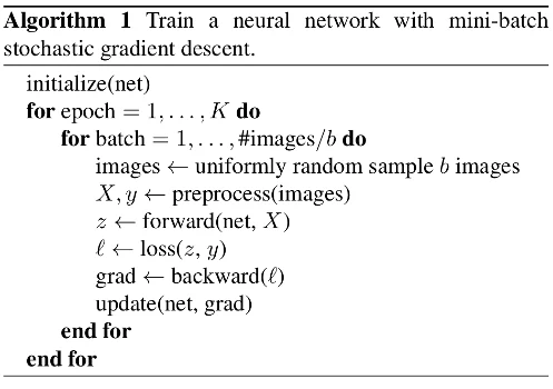
This section focuses on how to train a model. As an introduction, the authors remind us of the mini-batch stochastic gradient descent algorithm.
2.1. Baseline Training Procedure
In this section, they detail how they trained the models that will be used as a baseline in the paper.
- Randomly sample an image and decode it into 32-bit floating-point raw pixel values in [0, 255].
- Randomly crop a rectangular region whose aspect ratio is randomly sampled in [3/4, 4/3] and area randomly sampled in [8%, 100%], then resize the cropped region into a 224*224 square image.
- Flip horizontally with 0.5 probability.
- Scale hue, saturation, and brightness with coefficients uniformly drawn from [0.6, 1.4].
- Add PCA noise with a coefficient sampled from a normal distribution .
- Normalize RGB channels by subtracting 123.68, 116.779, 103.939, and dividing by 58.393, 57.12, 57.375, respectively.
The initialization is Xavier, NAG as the optimizer, 120 epochs, 8 NVIDIA Tesla V100, and a batch size of 256 (total). The learning rate is starting at 0.1 and is divided by 10 at the 30th, 60th, and 90th epochs. The models are trained on ImageNet Large Scale Visual Recognition Challenge dataset (ILSVRC2012).
2.2. Experiment Results
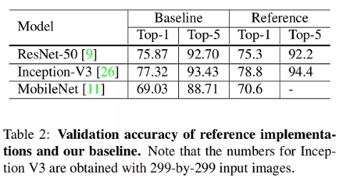
The authors evaluated ResNet-50, Inception-V3, and MobileNet-V1. The results for the baseline are given in Table 2 and compared with the reference (from the papers). Notice that ResNet-50 performs already slightly better but this is not the case for Inception-V3 and MobileNet-V1. This is due to the training procedure.
3. Efficient Training
Since the invention of that architecture, the hardware and especially the GPUs changed a lot. So the idea here is to review the training methods considering the new hardware.
3.1. Large-batch training
Linear scaling rate. Increasing the batch size reduces the noise in the gradient so we need to increase the learning rate. It is shown empirically that increasing the learning rate with the batch size is efficient. For a batch size of 256, the learning rate is set at 0.1 for ResNet-50. Then the learning rate is defined as equal to with b the batch size.
Learning rate warmup. Using a too large learning rate may result in numerical instability. The warmup heuristic is using a small learning rate at the beginning, this is called warmup. After few epochs (e.g. 5), considering the initial learning rate and the batch with , the learning rate is defined as .
Zero . We define a batch normalization in a ResNet architecture as . Both and are learnable parameters. In the zero heuristic, is initialized to 0. It is easier to train at the initial stage.
No bias decay. We apply a value decay only on the weights. The biases and and parameters in the batch normalization layer are left unregularized.
3.2. Low-precision training
Usually, all float variables are stored in a 32-bit floating-point (FP32). New Nvidia GPUs allow us to train neural networks with a mix of FP32 and FP16. The benefits are huge. For reference, the Nvidia Tesla v100 has 14 TFLOPS performance in FP32 and 100 TFLOPS in FP16. One of the methods consists in storing the values of the gradients and the activation function in FP16 and the weights in FP32.
3.3. Experiments Results
The batch size is 256 for the baseline and 1024 for the experiments ('Efficient" in table 3). Adding to that, they also used the heuristic described previously to train their models. The results are given in Table 3.
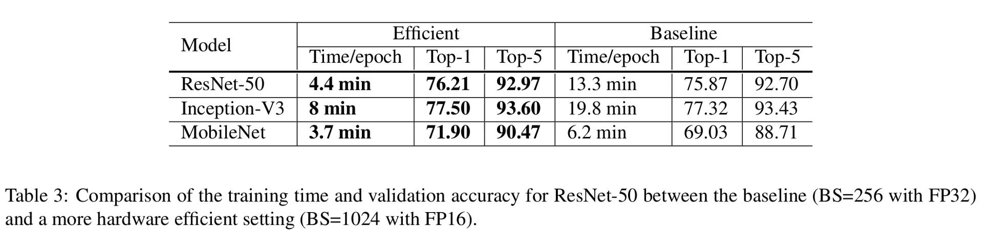
As we can see, the computation time is greatly reduced and the accuracy higher. For ResNet-50 from a top-1 accuracy of 75.87% and a computation time of 13.3 minutes per epochs, the authors obtain 4.4 minutes per epochs for 76.21% top-1 accuracy. The computation time is decreased by about 65% and the accuracy increased by 0.34%.
To understand which trick participated in the improvements, the authors did an ablation study on ResNet-50. The results are given in Table 4.
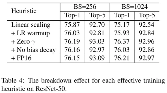
Increasing the batch size from 256 to 1024 by using linear scaling alone decreases the accuracy by 0.9%. The counterpart of this is that it accelerates significantly the training time as shown previously in Table 3. But the other heuristic raises again the accuracy from 75.27% top-1 accuracy in the case of batch size 1024 to 76.21%.
| BS=256 | BS=256 | BS=1024 | BS=1024 | |
|---|---|---|---|---|
| Heuristic | delta Top-1 | delta Top-5 | delta Top-1 | delta Top-5 |
| Linear scaling | 0.00 | 0.00 | 0.00 | 0.00 |
| + LR warmup | -0.16 | +0.11 | +0.76 | +0.30 |
| + Zero | +0.16 | +0.22 | +0.44 | +0.12 |
| + No bias decay | -0.03 | -0.06 | -0.34 | -0.10 |
| + FP16 | -0.01 | +0.12 | +0.18 | +0.11 |
table 4.1: Table 4 analysis
Table 4.1 present another format for the results given in table 4. There are a few things to notice. First, the contribution of the heuristics is different for a batch size of 256 and 1024. Same observation for the top-1 accuracy and the top-5. This suggests that those tricks do not necessarily generalize. Also, the no bias decay heuristic contributes negatively in all cases. It is mentioned in section 3.2 that this avoids overfitting though.
4. Model Tweaks
Here the authors analyze the architecture of ResNet-50 itself.
4.1. ResNet Architecture
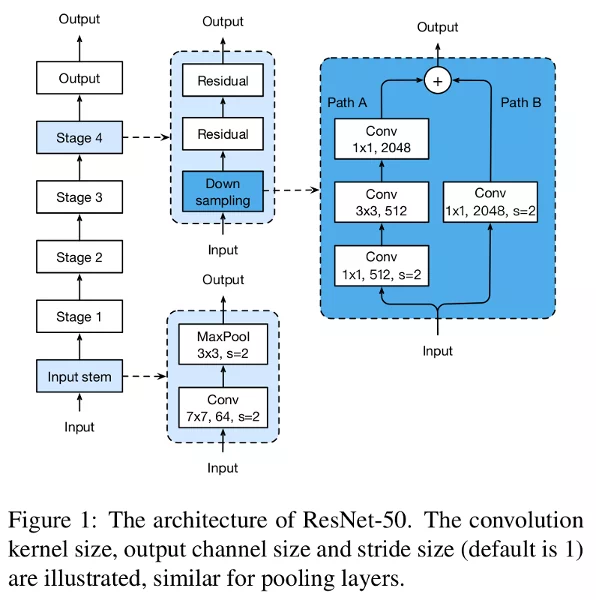
The vanilla architecture is given in figure 1 and explained in this section.
4.2. ResNet Tweaks
Previous tweaks are reviewed in the custom architecture is called ResNet-B and the second one ResNet-C. The authors propose new ones in the ResNet-D.
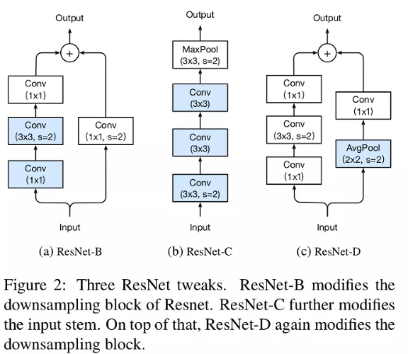
ResNet-B. Switch the strides' size of the first two convolutions in path A (figure 2a). Doing so, no information is ignored. This trick is implemented in the PyTorch implementation of ResNet.
ResNet-C. The computational cost of a convolution being quadratic to the kernel width or height, a 7x7 convolution is 5.4 times more expensive than a 3x3. So they replace the 7x7 convolutions with 3 3x3 (figure 2b).
ResNet-D. Similar to ResNet-B, the convolution in path B (figure 1) ignores 75% of the input feature maps. Empirically they found adding a 2x2 average pooling layer with a stride 2 before the convolution improves the accuracy without impacting too much the computational cost. This tweak is illustrated in figure 2c.
4.3. Experiment Results
Table 5 is giving the evaluation of the 3 custom architectures described previously. The batch size is 1024 and the precision is FP16.
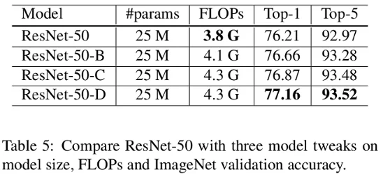
We can see that the ResNet-50-D is the most accurate with a top-1 accuracy of 77.16% compared to 76.21% of the vanilla architecture. The computational cost slightly (15%) increased though. The authors claim that in practice ResNet-50-D is only 3% slower than the vanilla one.
5. Training Refinements
5.1. Cosine Learning Rate Decay
Instead of using an exponential learning rate decay, previous work proposed a cosine decay.
Where is the initial learning rate. A comparison with the step decay is given in figure 3.
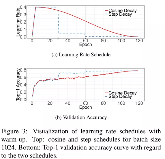
The cosine learning rate decay potentially improves the training progress.
5.2. Label Smoothing
Using softmax encourages the output scores of the model to be dramatically distinctive, which potentially leads to overfitting. The idea of label smoothing was proposed in inception-v2. It encourages a finite output from the fully connected layer (the last one) and can generalize better.
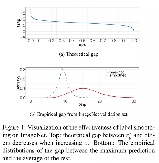
In figure 4a, the authors calculated the gap between the maximum prediction value and the average of the rest. Here the theoretical gap is around 9.1. In figure 4b we can see that the smoothed labels are denser around 9-10. This indicates that label smoothing allows fewer extreme values.
5.3. Knowledge Distillation
In knowledge distillation, we use a teacher model to help train the student model. The teacher model is usually a pre-trained model with higher accuracy and the student is learning by imitation. By using a specific loss function and the output of the teacher and student model, we can train the student model.
5.4. Mixup Training
Mixup is a replacement for classical data augmentation. Each image (and its label) is randomly linearly interpolated with a weighted different random image.
With a random number following the beta distribution.
5.5. Experiment Results
For the label smoothing . The distillation temperature . For the teacher, ResNet-152-D is used with the cosine learning rate decay, label smoothing is also used for the teacher, and mixup for the data augmentation. The number of epochs is increased from 120 to 200 because of the mixup. It requires more epochs to converge better.
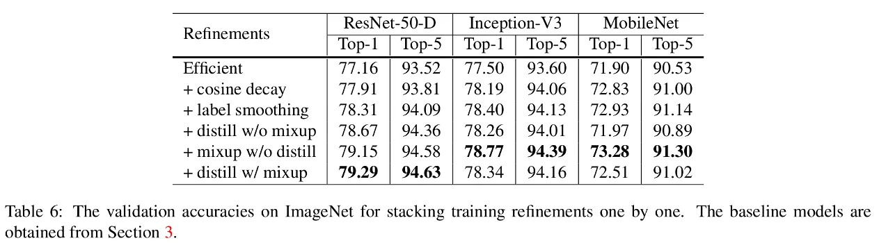
In table 6, the authors are showing that their work can be applied to other models. The model labeled "Efficient" is the one from table 5. The only difference is the knowledge distillation that doesn't work well on Inception-V3 and MobileNet. Their hypothesis is that because they use a different model for the teacher and the student. They also tested if their tricks apply to other datasets.
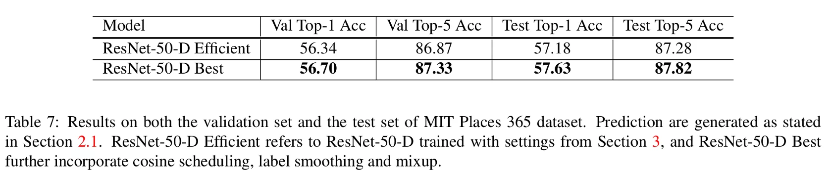
In table 7, they applied their models on MIT Places 365. The refinements improved consistently the accuracy.
6. Transfer Learning
In this section, they investigate how the refinements influence transfer learning.
6.1. Object Detection
For object detection, they used PASCAL VOC for the dataset and Faster-RCNN with refinements from Detectron such as linear warmup and long training schedule. The backbone is replaced with their models. The mean AP is reported in table 8.
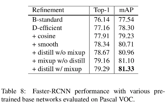
As expected, the model with the higher (top-1) accuracy is leading to the higher mAP and outperforming the standard model (faster-RCNN with ResNet-50-B as the backbone) by 4%.
6.2. Semantic Segmentation
For this task, they used FCN and trained it on ADE20K. They also replaced the backbone with their models.
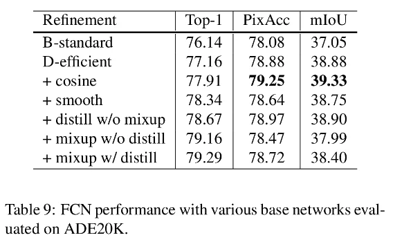
The results are reported in table 9. Those results are a bit more contrastive here. The authors hypothesize that the prediction at the pixel level is degraded by the label smoothing, distillation, and mixup. It blurs pixel-level information.
7. Conclusion
In this work, the authors surveyed several tricks that individually are not very interesting. But putting all together, they bring a very good accuracy improvement and allow to use of mixed precision. They also showed that these tricks apply to other models like Inception-V3 and MobileNet.