Framework for unsupervised learning in computer vision
tasks.

1. Introduction

With the democratization of deep learning, we came from hand-crafted features to models that learn those features. But data efficiency is still a challenge.

Learning a high-level representation from data that would be useful for any type of task is something very difficult and we don't even know what is the ideal representation.

One common strategy is to predict future, missing, or contextual information. This intuition is coming from other different fields such as neuroscience, signal processing, etc. The authors of the paper are hypothesizing that this approach is the key to extracting conditionally dependent values of the same high-level latent representation. Representations that would be generalizable.

Therefore, in this paper, the authors propose to:

compress high dimensional data into compact embedding space
then using auto-regressive models to make predictions many steps in the future

2. Contrastive Predicting Coding

2.1. Motivation and Intuitions

The intuition behind this paper is quite simple: by predicting far in the future, we can learn more global and meaningful structures instead of smaller irrelevant details. Take a painting as an example, if you are very close, you will see all the small details like cracks, but those details are not relevant to the work itself. By taking a step back, you avoid catching what would be considered noise. Figure 1 is showing this idea.

Uni-modal losses as generative models fail at modeling high dimensional data because they ignore the context c. Also, considering that an image may contain thousands of bits of information compared to a few bits for class labels for example suggests that modeling p(x|c) is may not be optimal. From this comes the idea of using more compact representations and looking at the common information between the future ( target x) and the present (context c).

I(x;c)= \sum_{x,c}p(x,c) \log \frac{p(x,c)}{p(x)} \tag{1}

The equation (1) represents the Mutual Information between $x$ and $c$ that we want to maximize. By doing so, we extract the underlying latent variables the inputs have in common.

Indeed, the mutual information is given by $I(x;c)=\sum_{x,c} \frac{p(x,c)}{p(x)p( c)}$ . The joint density function can be written as $p(x,c)=p(x|c).p( c)$ with $p(x|c)$ the conditional distribution. Then we can write (1).

2.2. Contrastive Predictive Coding

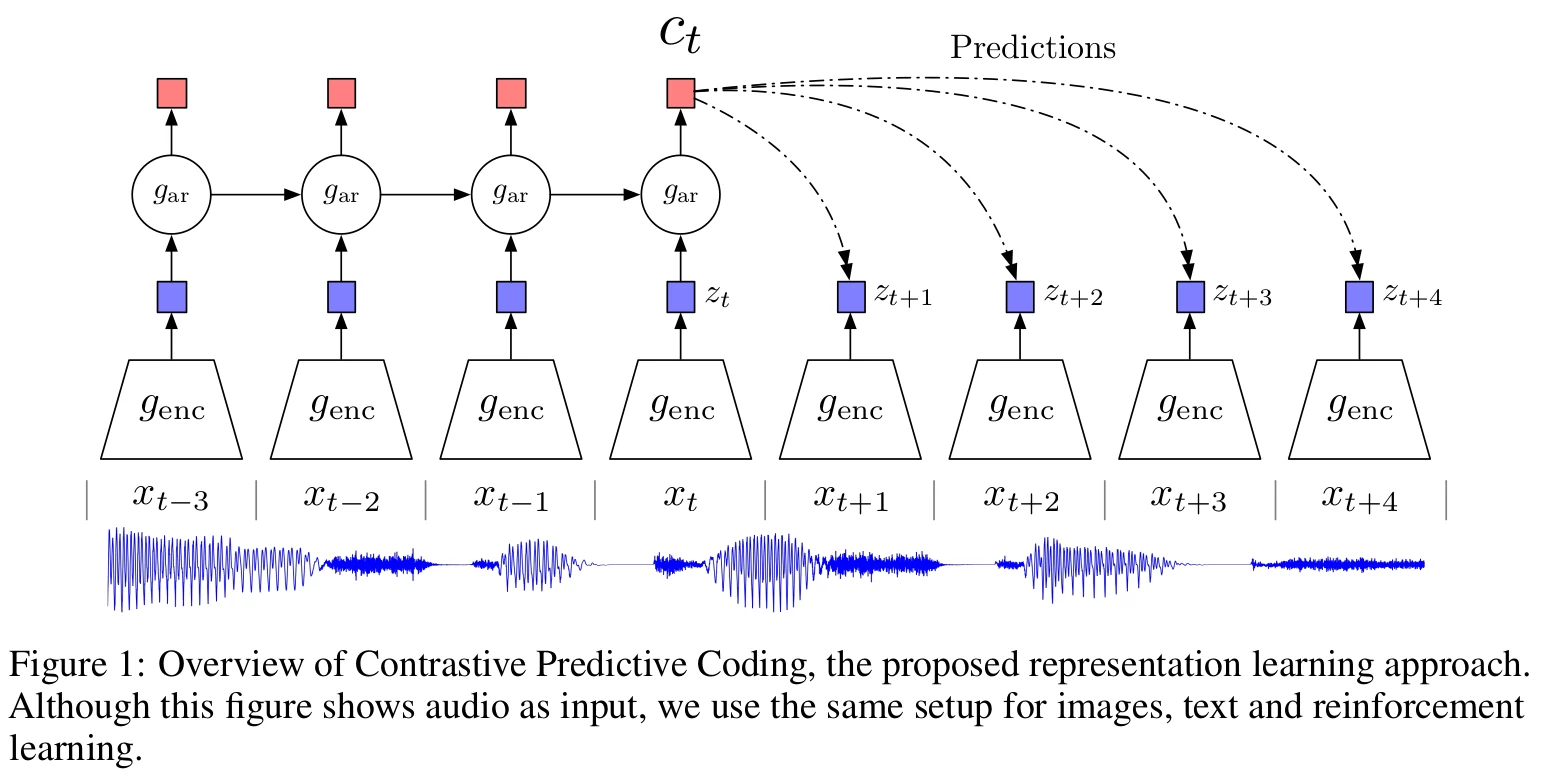
As we can see on the figure 1, the general framework consists of:

A non-linear encoder $g_{enc}$ maps the input sequence $x*t$ to a sequence of latent representation $z_t = g * { enc } (x_t)$ .
Then an autoregressive model $g* {ar}$ summarizes all $z* {\leq t}$ and produces a context $c*t = g * {ar} (z\_ {\leq t})$
A density ratio is modeled (they don't predict directly $x \_ {t+3}$ )

f _ k(x _ {t+k},c _ t)= exp(z _ {t+k}^T W _ k c _ t) \tag{2}

The log-bilinear model, given a context, predicts the representation for the next entity by linearly combining the representations of the contexts c. The authors add that the linear transformation $W_k^T c_t$ can be replaced by non-linear models like neural nets.

Finally, they infer $z \_ {t+k}$ with an encoder and by using techniques such as Noise-Contrastive Estimation (NCE) and Importance Sampling based on comparing the target value with randomly sampled negative values on the density ratio.

2.3. InfoNCE Loss and Mutual Information Estimation

The encoder and autoregressive model are trained together using a loss function based on NCE. Just some words about NCE, it is used for example in Word2Vec (a variation of NCE). The idea is that using a simple cross-entropy to predict the next word is inefficient since the number of classes (words) is huge. Instead, the problem is converted into a binary classification of good/bad. In this case, they call their loss function infoNCE. For each $c_t$ , the model has to predict among $X = {x_1, .... , x_N }$ which $x$ is the true one (the sample contains only 1 true).

\mathcal{L} _ N = - \underset{X}{\mathbb{E}} \left[ \log \frac{f _ k(x _ {t+k}, c _ t)}{\sum_{x _ j \in X}f _ k(x _ j,c _ t)} \right] \tag{3}

The authors are showing the density ratio from (2) is proportional to $\frac{}{}$ by looking at the optimal value of this loss function. Which confirms its usage.

Contrastive losses and predictive coding were already used in different ways but not combined (to make contrastive predictive coding, CPC).

3. Experiments

The authors experimented on 4 topics: audio, NLP, vision, and reinforcement learning.

3.1. Audio

For this first batch of experiments, the authors used 100 hours of the LibriSpeech dataset. It contains speech from 251 different speakers and is downloadable from the Google Drive's authors (link in the paper). They focus on 2 tasks to analyze their model, speaker classification and phone (a phone is any distinct speech sound or gesture, regardless of whether the exact sound is critical to the meanings of words, wiki) classification.

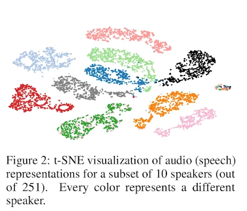
Figure 2 shows how discriminatory is the embedding for the speakers. Indeed we can see that the clusters are mostly clearly separable.

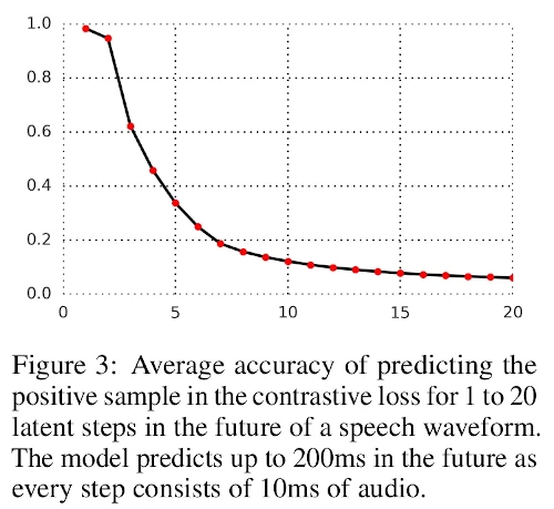
Figure 3 is showing the accuracy (vertical axis) of the model to predict future steps (horizontal axis), from 1 to 20 time steps ahead. As we can see, the task is becoming very difficult for many timesteps but doable for near future steps.

Then they extracted the embedding ( $c$ , outputs of $g_ {ar}$ of 256 dimensions) after training their model and trained a new multi-class linear logistic regression classifier. The top of table 1 is showing the results.

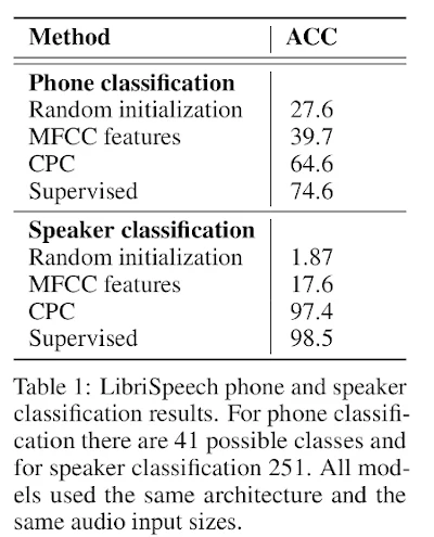
Random initialization is the authors' model without training, MFCC features are the Mel Frequency Cepstral Coefficient commonly used in speech and speaker recognition and supervised is the same model as CPC but trained end-to-end in a supervised way. As we can see, CPC is 10% under the supervised model. This means that the model is not using its full potential. And the accuracy is way higher than the traditional MFCC. As we mentioned, the authors used a linear classifier on top of their model but they noticed that some features information encoded in the model were not linearly accessible. By using a neural net with 1 hidden layer they could increase the model accuracy from 64.6 to 72.5%. Regarding the speaker classification (in table 1 still), the is way better. The accuracy of the CPC model is very close to the fully supervised model (97.4% to 98.5%). and far from the MFCC features. This is coherent with figure 2.

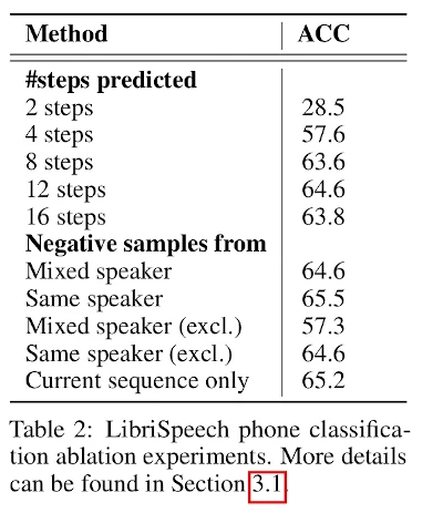
Table 2 shows an ablation study. In the top part, the authors study the number of optimal steps. 12 steps seem to be optimal. Then the analyze which strategy is the best regarding the negative samples (explained in 2.3.).

3.2. Vision

In these experiments, the authors used ImageNet. The framework is easier to understand for the images I felt. The figure 4 is describing it.

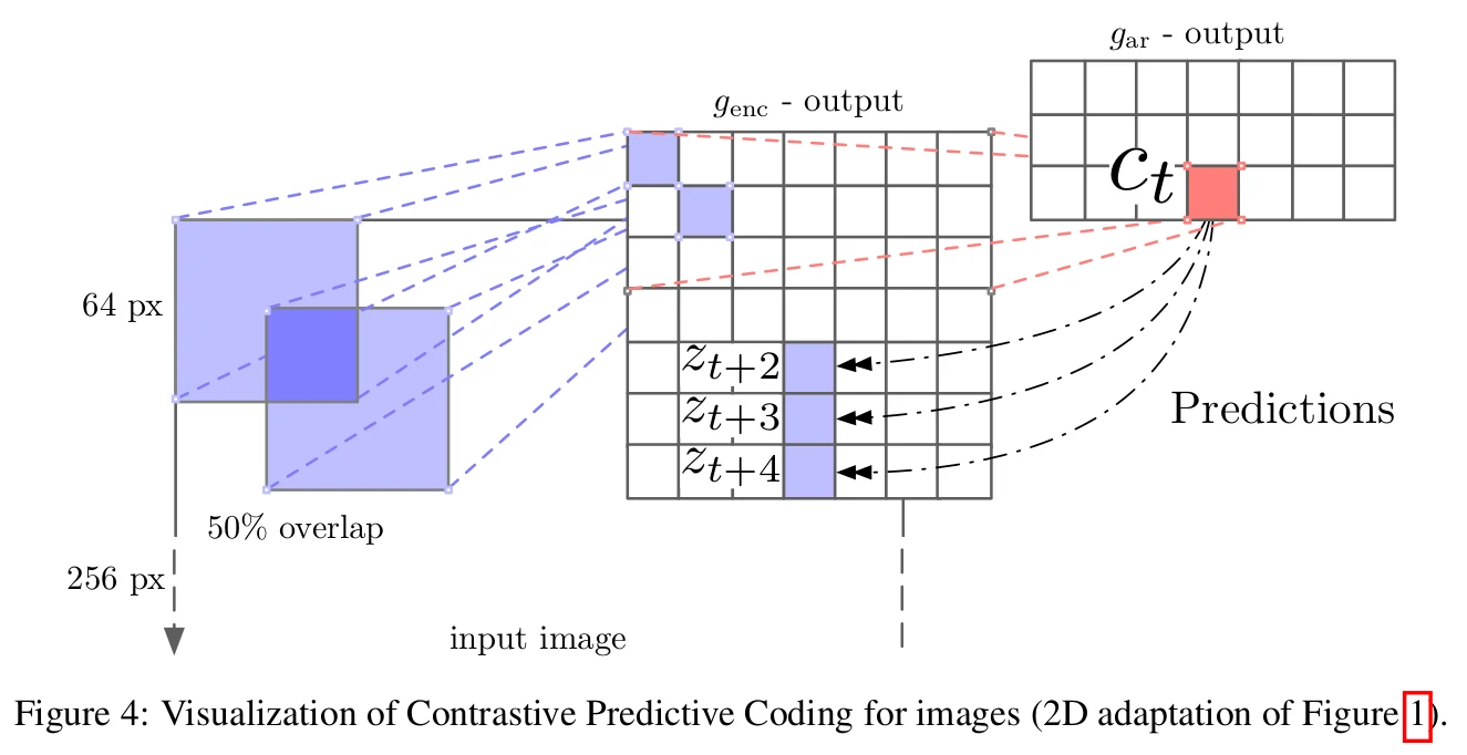
From the 256x256 initial images, they:

Extract a 7x7 grid of 64x64 crops with 32 pixels overlap
Each crop is encoded by a ResNet-v2-101 encoder. The output is a 1024 dimensions vector per 64x64 crops
This result in a 7x7x1024 tensor
A PixelCNN-style autoregressive model is used to make the predictions top-to-bottom
Tables 3 and 4 show the top-1 and top-5 (resp.) classification accuracies compared with the SOTA.

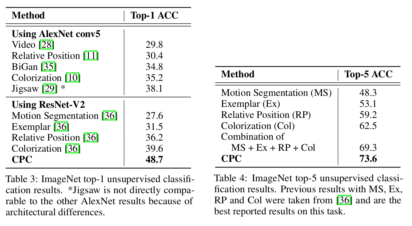
CPC improves by 9% the top-1 accuracy and 4% the top-5.

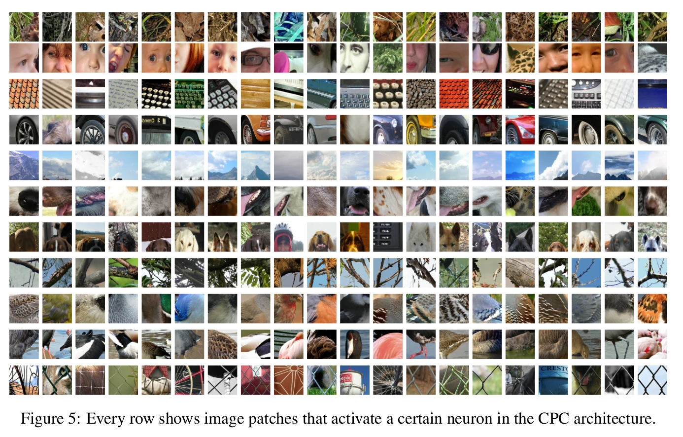
Figure 6 shows the patches where some neurons were activated. We can notice that these patches look quite relevant. This indicates that the framework is helping the model to learn some very meaningful patterns.

3.3. Natural Language

Here the unsupervised model is trained on the BookCorpus dataset. The CPC model is evaluated as a feature extractor (like in the previous experiments) by using CPC representations for a set of classification tasks. The tasks are movie review sentiment (MR), customer product reviews (CR), subjectivity/objectivity (Subj), opinion polarity (MPQA), and question-type classification (TREC). As before, a simple logistic regression classifier is trained on the feature extractor (CPC).

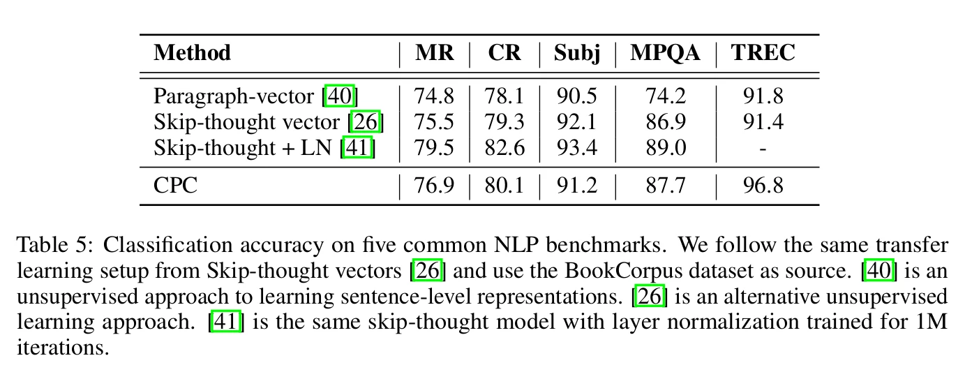
The results are shown in Table 5. The authors comment that the accuracy is close to the Skip-thought model but faster to train since Skip-thought is using a powerful LSTM. Also, the initial dataset might not be optimal.

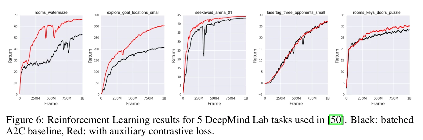
3.4. Reinforcement Learning

The model is tested on 5 3D environments of DeepMind Lab: rooms-waternaze, explore-goal-locations-small, seekavoid=arena-01, lasertag-three-opponents-small, and rooms-keys-doors-puzzle. This case differs a bit from the previous ones. The authors used the standard batched A2C agent and added CPC as an auxiliary loss. Figure 6 shows that on 4 of 5 of the performance of the games of the agent improves significantly.

4. Conclusion

The authors introduced CPC, which is quite promising but has to be improved. For example, even though the method is said to be unsupervised, we still need to train a classifier on top but annotated data. Also, the final accuracy is not necessarily the best when compared to supervised methods.